

Executive Overview: The Invisible Architecture Governing Modern AI
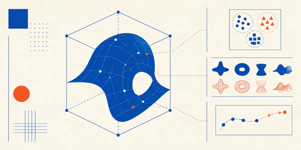
Behind every state-of-the-art artificial intelligence system—from natural language processors and diffusion-based image generators to high-throughput recommendation engines—lies an invisible, highly structured mathematical coordinate system known as the latent space.
At its core, a latent space is a low-dimensional, dense numerical representation of complex, high-dimensional real-world data. Raw information, whether presented as millions of image pixels, high-frequency audio waveforms, or intricate customer behavior logs, is inherently unwieldy and filled with noise. Machine learning models function by abstracting this unstructured chaos into a compressed vector space where semantically related concepts are mapped close together, and irrelevant variations are systematically discarded.
       +-------------------------------------------------------+
       |                 RAW HIGH-DIMENSIONAL DATA             |
       |  (Millions of Pixels, Audio Samples, Behavioral Logs)  |
       +-------------------------------------------------------+
                                   |
                                   v
                      +-------------------------+
                      |    ENCODER / MAPPER     |
                      | (PCA, VAE, Transformer) |
                      +-------------------------+
                                   |
                                   v
       +-------------------------------------------------------+
       |                     LATENT SPACE                      |
       |   (Dense, Low-Dimensional Geometric Representations)  |
       +-------------------------------------------------------+
             /                     |
            /                      |
           v                       v                       v
+--------------------+   +--------------------+   +--------------------+
|  DESCRIPTIVE ROLE  |   |  GENERATIVE ROLE   |   |  PREDICTIVE ROLE   |
| (Dimensionality    |   | (Interpolation &   |   | (Vector Search &   |
|  Reduction &       |   |  Novel Synthesis)  |   |  Classification)   |
|  Feature Mapping)  |   |                    |   |                    |
+--------------------+   +--------------------+   +--------------------+
Understanding how latent spaces operate is essential for comprehending modern computational intelligence. These mathematical spaces perform three fundamental functions across artificial intelligence architectures:
- Descriptive: Structuring, disentangling, and summarizing raw inputs into core semantic features.
- Generative: Serving as continuous mathematical canvases from which novel data instances can be sampled and synthesized.
- Predictive: Enabling geometric similarity calculations, semantic retrieval, and high-accuracy classification.
Detailed Chronology and Functional Taxonomy of Latent Spaces
The evolution of latent spaces traces the trajectory of machine learning itself—transitioning from linear algebraic transformations used in late 20th-century statistics to non-linear neural representations that power today’s foundation models.
               HISTORICAL EVOLUTION OF LATENT REPRESENTATIONS

  1900s-1980s: Linear Subspaces
  [PCA / SVD] ---> Linear projections, variance preservation

  1990s-2000s: Manifold Learning
  [t-SNE / LLE / Isomap] ---> Non-linear local distance preservation

  2010s: Neural Encoders & Deep Latent Spaces
  [VAEs / GANs / Autoencoders] ---> Continuous probabilistic distributions & manifolds

  2020s-Present: Multimodal Foundation Spaces
  [Transformers / CLIP / Diffusion] ---> Alignment of heterogeneous data modalities
1. The Descriptive Role: Structural Compression and Feature Disentanglement
The primary challenge in classical and deep learning is the "curse of dimensionality." High-dimensional inputs contain extensive redundancy. For instance, a $1024 times 1024$ pixel color image occupies over 3 million numeric channels, yet only a fraction of those pixels define the core subject.
The descriptive role of a latent space involves transforming raw inputs into a compressed numerical format that isolates latent variables—the underlying drivers of variation in data. In portrait processing, these variables might correspond to lighting conditions, facial geometry, or pose angle.
Classical Linear Compression via Principal Component Analysis (PCA)
Before deep neural networks dominated feature learning, linear techniques like Principal Component Analysis (PCA) served as the standard for isolating latent directions. PCA identifies orthogonal axes (principal components) along which the variance of the data is maximized, projecting high-dimensional arrays into lower dimensions while minimizing information loss.
The following Python example illustrates how a three-dimensional dataset can be reduced to a two-dimensional latent space:
import numpy as np
from sklearn.decomposition import PCA

# High-dimensional input: 3 samples across 3 measured features
raw_data = np.array([
    [1.1, 2.2, 3.3],
    [1.0, 2.1, 3.1],
    [8.1, 9.2, 9.9]
])

# Initialize PCA to compress data into a 2D Latent Representation
pca = PCA(n_components=2)
latent_space_map = pca.fit_transform(raw_data)

print("--- Descriptive Latent Space Matrix ---")
print(latent_space_map)
print("nExplained Variance Ratio:", pca.explained_variance_ratio_)
Output:
--- Descriptive Latent Space Matrix ---
[[-3.88962445  0.04396345]
 [-4.11856576 -0.04313346]
 [ 8.00819021 -0.00082999]]

Explained Variance Ratio: [0.99974241 0.00025759]
In this system, the first component captures over 99.9% of the total variance, successfully reducing the input dimension while preserving the essential structure separating the first two data points from the third.
2. The Generative Role: Latent Manifolds as Synthetic Canvases
Once a model establishes a structured latent space, that space can function as a generative canvas. Rather than simply mapping inputs into vectors, the model can navigate the continuous vector space to synthesize brand-new data points.
Generative architectures—such as Variational Autoencoders (VAEs), Generative Adversarial Networks (GANs), and Latent Diffusion Models (LDMs)—depend on the continuity of the latent manifold. Because the space is continuous, traversing the distance between vector $mathbfz_A$ and vector $mathbfz_B$ produces smooth transitions in the output space.
       Latent Point A (z_A)  ==============>  Latent Point B (z_B)
         [Vector State A]                       [Vector State B]
                                   |
                                   v
                 Interpolation Point (0.5 * z_A + 0.5 * z_B)
                                   |
                                   v
                    Decoder / Inverse Transformation
                                   |
                                   v
                    Synthesized Data Instance (Output)
By interpolating between known vectors or sampling from learned probability distributions, models generate novel images, audio, or text representations that align with the training distribution.
Latent Space Vector Interpolation Implementation
The script below demonstrates vector interpolation within a transformed latent space, decoding a synthetic vector back into the original input domain:
# Select two distant points within the learned 2D latent space
point_a = latent_space_map[0]  # Vector representing Sample 1
point_b = latent_space_map[2]  # Vector representing Sample 3

# Mathematical Interpolation: Calculate the geometric midpoint
generated_latent_point = 0.5 * point_a + 0.5 * point_b

# Reshape for transformation compatibility
generated_latent_point = generated_latent_point.reshape(1, -1)

# Decode the synthetic latent coordinate back into the original 3D domain
generated_raw_data = pca.inverse_transform(generated_latent_point)

print("--- Synthetic Latent Point Coordinates ---")
print(generated_latent_point)
print("n--- Decoded Synthetic Data Point (Original Domain) ---")
print(generated_raw_data)
Output:
--- Synthetic Latent Point Coordinates ---
[[ 2.05928288  0.02156673]]

--- Decoded Synthetic Data Point (Original Domain) ---
[[4.6 5.7 6.6]]
This mathematical technique forms the basis of modern generative models. For instance, adjusting specific directional vectors in an image model’s latent space allows for targeted edits, such as modifying age, lighting, or expression, while preserving overall image consistency.
3. The Predictive Role: Semantic Geometry and Similarity Systems
The third primary function of latent spaces is predictive analysis. When high-dimensional data is mapped into a well-structured latent space, geometric distance directly mirrors semantic similarity. Data items sharing conceptual traits cluster together, while dissimilar items are separated by larger vector distances.
                   SIMILARITY MEASUREMENT IN LATENT SPACE

                           +Y |           * Item B (0.1, 0.9)
                              |          /
                              |         / Angle theta (Cosine Similarity)
                              |        /
                              |       * Query Point (0.0, 1.0)
                              |
     -------------------------+------------------------- +X
                              |
                              |
                              |   * Item A (-3.8, 0.04)
                              |-Y
This structural property powers modern recommendation engines, facial recognition systems, and Retrieval-Augmented Generation (RAG) pipelines. By measuring directional alignments—such as through Cosine Similarity—models can quickly identify related entries across large-scale vector databases.
Predictive Similarity Calculation Implementation
The Python example below demonstrates how cosine similarity can be calculated within a latent space to match an incoming query vector against existing dataset records:
from sklearn.metrics.pairwise import cosine_similarity

# Define a new query point within the latent coordinate framework
new_item_latent = np.array([[0.0, 1.0]])

# Compute pairwise cosine similarity scores against reference coordinates
similarity_scores = cosine_similarity(new_item_latent, latent_space_map)

print("--- Predictive Similarity Vector ---")
print(similarity_scores)

# Identify the closest match by index
best_match_idx = np.argmax(similarity_scores)
print(f"nClosest Semantic Index: best_match_idx with score similarity_scores[0][best_match_idx]:.6f")
Output:
--- Predictive Similarity Vector ---
[[ 0.01130203 -0.01047236 -0.00010364]]

Closest Semantic Index: 0 with score 0.011302
In enterprise settings, vector search engines like Pinecone, Milvus, and Qdrant execute these operations over millions of high-dimensional dense vectors in milliseconds, providing the backend retrieval mechanics for modern LLM architectures.
Supporting Context, Mathematical Foundations, and Industry Metrics
To evaluate latent space efficiency across applications, researchers and engineers rely on core mathematical metrics and operational trade-offs.
| Metric / Dimension | Mathematical Formulation | Primary Application | Target Optimization Goal |
|---|---|---|---|
| Cosine Similarity | $cos(theta) = fracmathbfu cdot mathbfv$ | Semantic text search, RAG, recommendation matching | Maximize alignment ($rightarrow 1.0$) for relevant items |
| Euclidean Distance ($L_2$) | $d(mathbfu, mathbfv) = sqrtsum_i=1^n (u_i – v_i)^2$ | Clustering, spatial embeddings, facial verification | Minimize distance for identical entities |
| Explained Variance | $fracsum_i=1^k lambdaisumj=1^p lambda_j$ | Linear dimensionality reduction (PCA) | Preserve maximum variance using minimal dimensions ($k ll p$) |
| Kullback-Leibler (KL) Divergence | $D_KL(P parallel Q) = int p(x) log fracp(x)q(x) dx$ | Variational Autoencoders (VAEs) | Regularize latent spaces against standard normal distributions |
| Fréchet Inception Distance (FID) | $|mu_r – mu_g|^2 + textTr(Sigma_r + Sigma_g – 2(Sigma_rSigma_g)^1/2)$ | Evaluation of generative image quality | Minimize discrepancy between real and generated distributions |
Topological Vulnerabilities: Representation Collapse and Anisotropy
Despite their capabilities, latent space implementations present technical challenges:
- Posterior Collapse: Often encountered in VAE training, this occurs when the model’s decoder ignores the latent variable entirely, rendering the latent representation uninformative.
- Anisotropy: High-dimensional embedding spaces, particularly in Large Language Models, often compress vectors into a narrow cone within the vector space. This spatial concentration reduces expressiveness and distorts distance-based similarity metrics.
- Curse of Dimensionality in Vector Indexing: As latent dimensions expand (e.g., beyond 1,536 dimensions), standard metric operations face computational bottlenecks. This requires specialized approximate nearest neighbor (ANN) indexing algorithms, such as Hierarchical Navigable Small World (HNSW) graphs.
Industry Consensus and Research Perspectives
Leading artificial intelligence researchers increasingly view latent space design as a central component in achieving advanced AI capabilities.
"The future of AI lies in Joint Embedding Predictive Architectures (JEPA). Rather than trying to predict every pixel in an image or every token in a sentence, systems must learn to predict abstractions within a joint latent space. This eliminates noise and allows models to focus on essential semantic structure."
— Yann LeCun, Chief AI Scientist at Meta and Turing Award Laureate
This perspective highlights an industry-wide transition away from processing surface-level inputs directly. Instead, research efforts are shifting toward operating within structured, abstract latent spaces.
"Representation learning is the primary reason deep neural networks succeed where hand-engineered models failed. By allowing the network to discover its own latent manifolds, we enable machines to capture complex, non-linear dependencies across diverse domains."
— Yoshua Bengio, Founder and Scientific Director of Mila
Future Outlook: Multimodal Alignment and Continuous Latent Architectures
The development of latent space architectures is moving toward universal multimodal alignment and continuous reasoning environments.
                      UNIFIED MULTIMODAL LATENT SPACE

      Text Inputs       Image Inputs      Audio Inputs      Video Inputs
     ("A blue car")     (Pixel Grid)      (Audio Wave)      (Video Frames)
                            |                 |                 /
                            |                 |                /
             v               v                 v               v
    +-----------------------------------------------------------------+
    |                UNIFIED MULTIMODAL LATENT SPACE                  |
    |      (Shared geometric coordinates across all data types)       |
    +-----------------------------------------------------------------+
                                     |
                                     v
                  +-------------------------------------+
                  |       Cross-Modal Generation        |
                  |  (Text-to-Video, Audio-to-3D, etc.) |
                  +-------------------------------------+
Key Trends Shaping the Field:
- Unified Cross-Modal Spaces: Models like OpenAI’s CLIP and ImageBind demonstrate that disparate data modalities (text, vision, audio, thermal data) can share a single, unified latent space. In these spaces, the text string "a dog barking" maps to the same geometric coordinates as an audio sample of a bark or a video clip of a dog.
- Continuous Reasoning Trajectories: Next-generation reasoning systems are moving beyond discrete text-token generation. Models are increasingly being trained to execute intermediate reasoning steps directly within continuous latent spaces, allowing for higher computational efficiency before generating final natural language outputs.
- Hyper-Dimensional Scale and Dedicated Hardware: Vector spaces are scaling in complexity, driving adoption of optimized hardware architectures (such as specialized tensor chips) and advanced vector database systems designed specifically for hyper-dimensional operations.
Ultimately, latent spaces serve as the primary mathematical abstraction enabling modern machine learning systems to process, generate, and reason over real-world data. By converting raw inputs into structured geometric coordinates, latent representations provide a unified framework that continues to drive advancements in artificial intelligence.
