

Executive Overview
In the high-stakes deployment of enterprise Large Language Models (LLMs), hardware efficiency is directly tied to financial viability. Thousands of high-performance graphics processing units (GPUs)—such as the NVIDIA H100 and A100—frequently operate at a fraction of their theoretical compute capacity. The root cause of this inefficiency lies in the mismatch between traditional deep learning batching methods and the unpredictable, autoregressive nature of generative AI workloads.
When processing LLM inference, an individual request might demand a five-token response, while another requires two thousand tokens. In traditional serving setups, GPUs spend substantial time waiting on memory transfers rather than executing compute operations. Because loading model weights from High Bandwidth Memory (HBM) into processing cores incurs high latency overhead, executing single requests sequentially leaves massive compute resources idle.
+-----------------------------------------------------------------------+
|                       GPU Execution Timeline                          |
+-----------------------------------------------------------------------+
| Single Request: [ Load Weights ] -> [ Process Token ] -> [ GPU IDLE ] |
|                                                                       |
| Batched Pass:    [ Load Weights ] -> [ Process K Requests Together ]   |
+-----------------------------------------------------------------------+
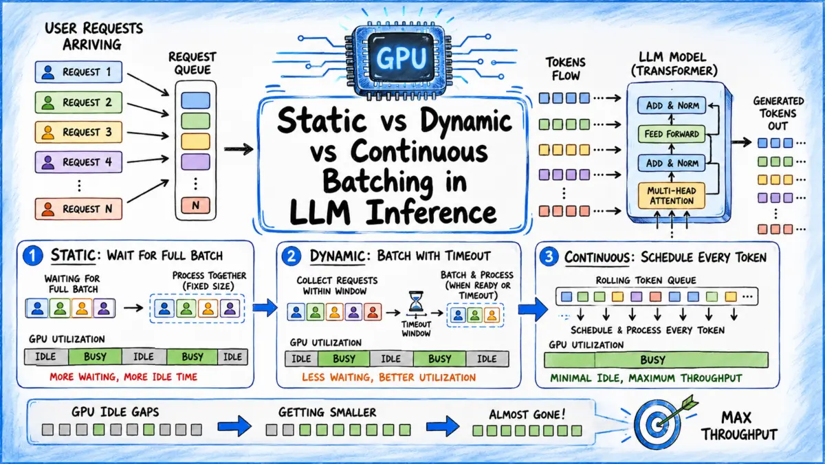
To resolve this bottleneck, software engineers and AI system architects have overhauled inference execution pipelines. The industry has migrated from basic Static Batching to time-bounded Dynamic Batching, and ultimately to iteration-level Continuous Batching (also referred to as in-flight batching).
This architectural shift moves scheduling away from coarse, request-level boundaries down to fine-grained, token-level decoding steps. Understanding these batching methodologies is critical for infrastructure architects seeking to maximize hardware throughput, reduce Time-to-First-Token (TTFT), and stabilize Inter-Token Latency (ITL) at scale.
Detailed Chronology: The Evolution of Inference Batching
+----------------------------------------------------------------------+
| EVOLUTION OF BATCHING PARADIGMS                                      |
|                                                                      |
|  1. STATIC BATCHING (Fixed Request Size)                             |
|     [Req 1: Token 1 2 3]                                             |
|     [Req 2: Token 1 2 3 4 5 6 7 8] -> Waiting for batch completion   |
|                                                                      |
|  2. DYNAMIC BATCHING (Timeout + Max Batch Size)                      |
|     [Timer Starts] -> Accumulate Requests -> Run Batch               |
|     (Padding wasted on unequal sequence lengths)                    |
|                                                                      |
|  3. CONTINUOUS BATCHING (Iteration-Level / In-Flight)                |
|     [Step 1: Req 1, Req 2, Req 3]                                    |
|     [Step 2: Req 1 finishes -> Freed] -> [Req 4 Inserted Immediately]|
+----------------------------------------------------------------------+
Phase 1: The Monolithic Era of Static Batching
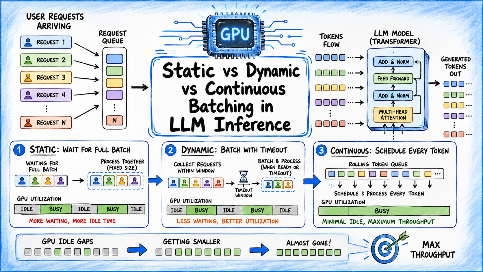
In the early stages of deep learning deployment, models primarily performed classification, regression, or single-pass feature extraction (e.g., ResNet, early BERT variants). Input tensor shapes were uniform or easily predictable. Systems relied on Static Batching, a mechanism wherein the inference server waits until a predefined number of requests ($N$) arrive in the queue before constructing a single monolithic tensor and firing a forward pass across the network.
While effective for offline, latency-tolerant workloads—such as overnight batch classification over millions of pre-stored records—static batching failed under live traffic conditions. If a batch size was set to 16, the 15th incoming request was forced to wait indefinitely in the queue until the 16th request materialized. Under sparse traffic, latency spiked significantly; under variable-length workloads, shorter requests were trapped until the longest request completed its entire generation loop.
Phase 2: The Service-Level Optimization of Dynamic Batching
To adapt static batching for production APIs, frameworks like Triton Inference Server and TorchServe introduced Dynamic Batching. This strategy preserved the premise of whole-request grouping but mitigated tail latencies by introducing a dual-trigger threshold: a maximum batch size combined with a timeout window ($Delta t$).
                      +-------------------+
                      | Incoming Request  |
                      +---------+---------+
                                |
                                v
                   +-------------------------+
                   | Queue & Start Timer Δt  |
                   +------------+------------+
                                |
             +------------------+------------------+
             |                                     |
             v                                     v
   [Batch Size Reached?]                 [Timeout Δt Expired?]
             |                                     |
             +------------------+------------------+
                                | YES
                                v
                   +-------------------------+
                   |   Trigger Forward Pass  |
                   +-------------------------+
Under dynamic batching, a timer initializes upon the arrival of the first request. If the batch reaches maximum capacity before the timer expires, the server immediately executes the batch. If traffic is low and the timer reaches its limit first, the server dispatches a smaller, partial batch.
While this design established an upper bound on initial queue latency, it suffered from severe inefficiencies when applied to generative autoregressive models. Because all sequences in a dynamic batch were bound to the same execution lifespan, shorter responses required extensive matrix padding (<PAD> tokens) to align with the longest sequence in the batch, causing substantial floating-point operation (FLOP) waste.
Phase 3: The Iteration-Level Revolution of Continuous Batching
The modern era of LLM serving began with the introduction of iteration-level scheduling, popularized by academic breakthroughs such as the Orca architecture (OSDI 2022) and subsequently industrialized by frameworks like vLLM, TensorRT-LLM, and Hugging Face Text Generation Inference (TGI).
Recognizing that LLM inference consists of distinct token-by-token generation iterations, Continuous Batching breaks the rigid request-level abstraction. Instead of treating a batch as an indivisible set of full requests, the scheduler operates at the level of individual token generation steps. At every iteration, sequences that reach their end-of-sequence (<EOS>) token are evicted from the active compute context immediately. The vacant execution slots are then backfilled on the very next step by newly arrived requests from the queue.
Supporting Context, Technical Mechanics & Metrics
To understand why continuous batching outpaces previous methodologies, one must examine the computational mechanics of LLM inference: the Prefill Phase and the Decode Phase.
+----------------------------------------------------------------------+
| INFERENCE PHASES                                                     |
|                                                                      |
| Prefill Phase (Prompt Processing):                                   |
| - Compute-Bound (High Arithmetic Intensity)                          |
| - Processes all prompt tokens in parallel via matrix-matrix multiplies|
|                                                                      |
| Decode Phase (Token Generation):                                     |
| - Memory-Bandwidth-Bound (Low Arithmetic Intensity)                  |
| - Generates one token at a time sequentially per active request       |
+----------------------------------------------------------------------+- The Prefill Phase (Compute-Bound): When a user sends a prompt, the model processes all input tokens simultaneously to compute the initial Key-Value (KV) cache. This phase exhibits high arithmetic intensity, fully saturating GPU Tensor Cores.
- The Decode Phase (Memory-Bandwidth-Bound): Generating output tokens happens sequentially. For every single token generated, the GPU must fetch the entire model parameters (tens or hundreds of gigabytes) from HBM into local SRAM. Here, arithmetic intensity is low; execution speed is dictated by memory bandwidth rather than raw compute speed.
Comparative Failure Analysis of Request-Level Batching
In static and dynamic batching, if Request A requires 10 output tokens and Request B requires 500 output tokens, both requests are locked into a single execution block for 500 steps.
Static / Dynamic Batching Execution Profile (Padding Overhead):
Req A (10 tokens):  [T1][T2]...[T10][PAD][PAD]...[PAD500] -> Wasted Compute & Memory
Req B (500 tokens): [T1][T2].....................[T500]

Continuous Batching Execution Profile (Dynamic Slot Allocation):
Slot 1: [Req A: T1..T10] -> [Evict] -> [Req C Prefill] -> [Req C Decode...]
Slot 2: [Req B: T1............................................T500]
This structural mismatch results in two major performance penalties:
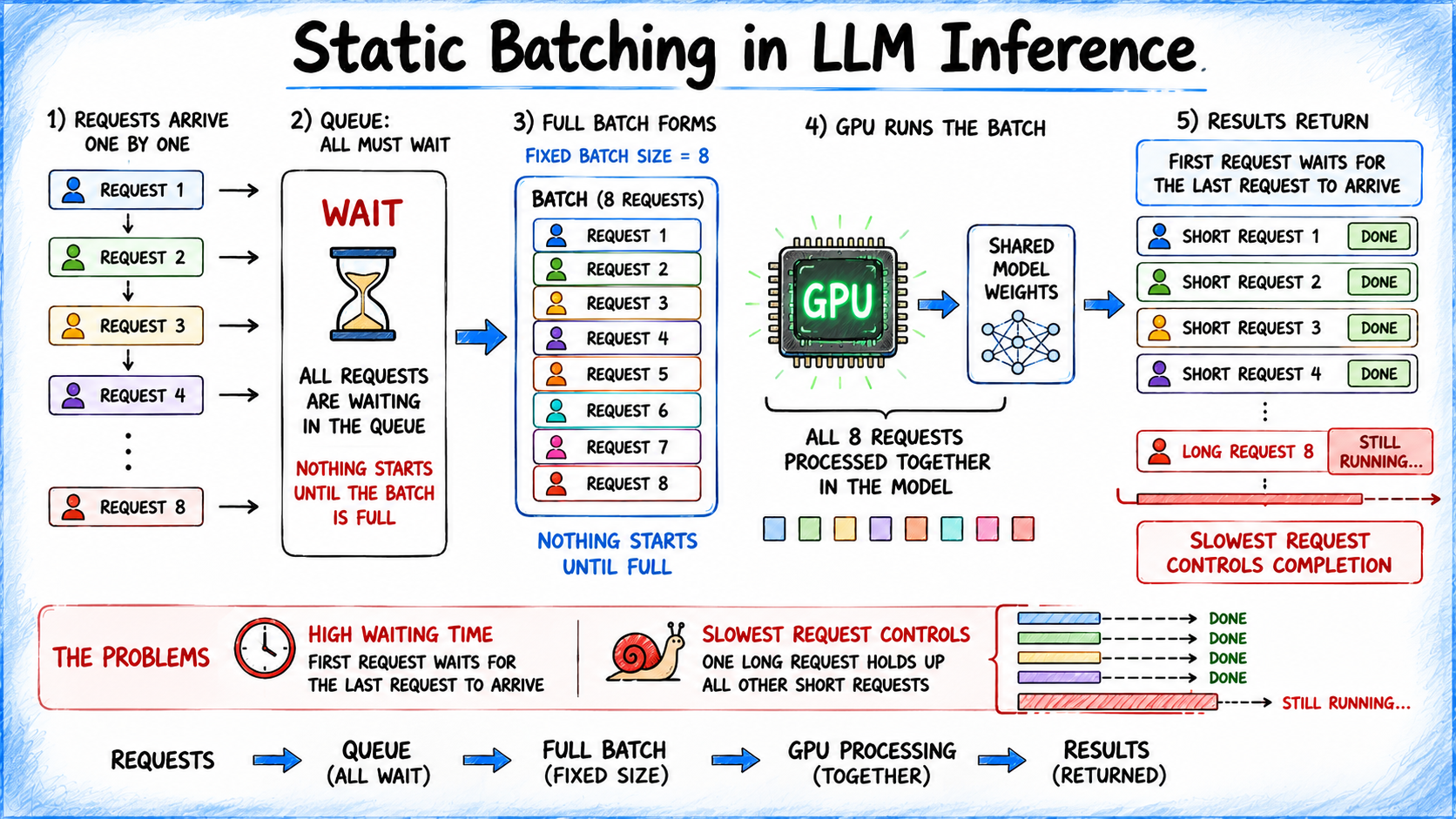
- Padding Overhead: Matrix multiplication requires rectangular tensor dimensions. Sequences shorter than the maximum length are padded with structural zeros, consuming memory and compute operations without generating value.
- Trailing Compute Waste (Straggler Problem): As shorter sequences finish, their slots remain vacant yet statically allocated within the running execution matrix until the single longest request finishes.
Continuous batching solves both issues by decoupling request boundaries. Through specialized memory allocation techniques such as PagedAttention—which manages the Key-Value (KV) cache in non-contiguous physical memory blocks similar to virtual memory in operating systems—continuous batching entirely eliminates structural padding.
Comprehensive Performance Comparison Matrix
| Metric / Dimension | Static Batching | Dynamic Batching | Continuous / In-Flight Batching |
|---|---|---|---|
| Scheduling Unit | Monolithic Request Group | Request Group + Time Constraint | Single Token Iteration Step |
| GPU Compute Utilization | Poor ($<20%$ in generative workloads) | Moderate ($30% – 50%$) | High ($70% – 90%+$) |
| Padding Waste | Severe | High | Zero (via non-contiguous memory management) |
| Time-to-First-Token (TTFT) | High (Dependent on queue fill) | Bounded by timeout parameter | Low (Prompts ingested on next iteration) |
| Inter-Token Latency (ITL) | Fixed by batch max-length | Fixed by batch max-length | Highly stable across active generation |
| Memory Management | Static contiguity requirement | Static contiguity requirement | Dynamic allocation (Paged KV Cache) |
| Optimal Use Case | Offline processing, static datasets | Fixed-length generation (e.g., SDXL) | Real-time, multi-tenant LLM serving APIs |
Official Statements & Industry Perspectives
The transition to continuous batching has driven architectural shifts across key enterprise framework maintainers and cloud providers:
NVIDIA Developer Documentation (TensorRT-LLM):
"In-flight batching (continuous batching) transforms how server resources are utilized. By processing requests at the step level rather than the request level, TensorRT-LLM minimizes idle Tensor Core cycles, delivering up to 4x throughput improvements over traditional dynamic batching on complex, mixed-length LLM workloads."Modular Engine Technical Architecture Overview:
"In multi-tenant LLM deployment, static request abstractions are fundamentally flawed. The execution runtime must treat sequence lengths as dynamic streams. Continuous batching, combined with advanced memory management, changes serving costs from linear scaling to logarithmic scaling under heavy concurrent request volumes."vLLM Core Engineering Group Insights:
"Traditional dynamic batchers could achieve high hardware utilization only by penalizing individual user response latency. PagedAttention combined with iteration-level continuous batching decoupled hardware utilization from request latency, proving that high throughput and minimal tail-latency can co-exist."
In benchmark analyses conducted across open-source inference engines, dynamic batching outperforms continuous batching in one edge scenario: light, single-tenant traffic with deterministic prompt lengths. When concurrent request counts fall to near zero, dynamic batching avoids the minor scheduling overhead incurred by an iteration-level engine, offering marginally lower absolute TTFT. However, under realistic enterprise concurrency (tens to thousands of concurrent streams), continuous batching routinely achieves $2times$ to $5times$ higher token throughput on identical GPU hardware topologies.
Future Outlook: Beyond Standard Continuous Batching
While continuous batching has established itself as the operational baseline for high-performance LLM deployment, modern production demands are pushing system architectures further. Modern inference stacks are evolving past pure continuous batching to resolve new bottlenecks introduced by heavy prefill loads.

+----------------------------------------------------------------------+
| EMERGING ARCHITECTURES                                               |
|                                                                      |
| 1. Chunked Prefills (e.g., Sarathi-Efficient):                       |
|    Splits massive prompt prefills into uniform chunks, preventing     |
|    long prompts from starving active token decode streams.           |
|                                                                      |
| 2. Prefill-Decode Disaggregation (PD-Disaggregation):               |
|    Allocates distinct GPU clusters exclusively to Prefill (Compute)  |
|    or Decode (Memory Bandwidth) stages, transferring KV caches over  |
|    high-speed interconnects (NVLink/InfiniBand).                     |
|                                                                      |
| 3. Speculative Decoding Integration:                                 |
|    Pairs small draft models with large target models inside the      |
|    continuous batching loop to generate multiple tokens per step.    |
+----------------------------------------------------------------------+
1. Chunked Prefills (Sarathi Architecture)
A remaining vulnerability of standard continuous batching occurs when a massive prompt (e.g., a 32,000-token document) enters the queue. Ingesting this prompt requires a large prefill computation step that blocks ongoing decoding iterations for existing requests, causing noticeable spikes in Inter-Token Latency (ITL).
To solve this, frameworks are adopting Chunked Prefills. Large prompt prefills are broken down into smaller chunks (e.g., 512 tokens) and piggybacked alongside routine decode iterations. This normalizes execution time across steps, maintaining stable inter-token generation speed while ingesting large contexts.
2. Prefill-Decode Disaggregation
Advanced production environments are beginning to physically isolate the prefill and decode stages onto separate hardware clusters:
- Prefill Nodes: Optimized with compute-heavy configurations (high Tensor Core count) to ingest context rapidly.
- Decode Nodes: Optimized for high memory bandwidth and capacity to manage massive KV caches across hundreds of concurrent streams.
In this architecture, continuous batching operates independently within the decode cluster, while high-speed interconnects (such as NVLink or InfiniBand) stream KV cache states directly from prefill nodes to decode nodes upon prompt completion.
3. Speculative Decoding Integration
Integrations of Speculative Decoding within continuous batching pipelines enable target LLMs to verify multiple candidate tokens generated by a smaller, faster draft model in a single execution step. Combining speculative decoding with iteration-level continuous batching allows inference engines to break through the memory bandwidth bottleneck, generating multiple output tokens per forward pass without sacrificing output quality.
Conclusion
The shift from static to continuous batching represents a fundamental evolution in AI infrastructure engineering. By discarding legacy, request-level assumptions in favor of iteration-level execution, systems architects have drastically closed the gap between theoretical hardware performance and real-world inference throughput.
As enterprise models continue to grow in parameters and context window lengths, mastering and deploying these batching paradigms remains essential for running efficient, scalable, and cost-effective AI serving infrastructures.
